Author: Owl

  • Excel VLOOKUP Function Guide: Basic Usage and XLOOKUP Comparison

    Have you ever needed to pull a customer’s email address from one sheet just by knowing their ID? Or match product prices across two different tables without manually scrolling and copy-pasting? This is exactly what VLOOKUP was built for — and once you understand it, you’ll wonder how you managed without it.

    In this guide, you’ll learn how to use VLOOKUP step by step, the most common mistakes that break it, and how the newer XLOOKUP function fixes those limitations.


    🔍 What Does VLOOKUP Actually Do?

    VLOOKUP stands for Vertical Lookup. It searches for a value in the first column of a range, then returns a value from a specified column to the right of it in that same row.

    Syntax:

    =VLOOKUP(lookup_value, table_array, col_index_num, [range_lookup])
    
    ArgumentWhat It Means
    lookup_valueThe value you’re searching for (e.g., a Customer ID)
    table_arrayThe full range containing your lookup data
    col_index_numWhich column (counting from the left, starting at 1) to pull the result from
    range_lookupFALSE for exact match (almost always what you want), TRUE for approximate match

    🛠️ Step 1: Set Up Your Lookup Table

    Make sure your data is structured with the value you’ll search by (e.g., Product ID) in the leftmost column of your range. VLOOKUP can only look to the right — it cannot search backward.

    🛠️ Step 2: Write the Formula

    1. Click the cell where you want the result to appear.
    2. Type =VLOOKUP(
    3. Select the cell containing the value you want to look up (e.g., A2).
    4. Select the full table range containing your data (e.g., Sheet2!A:D).
    5. Enter the column number to return (e.g., 3 for the third column in that range).
    6. Type FALSE for an exact match, then close the parenthesis and press Enter.

    Example:

    =VLOOKUP(A2, Sheet2!A:D, 3, FALSE)
    

    This looks up the value in A2, searches for it in the first column of Sheet2!A:D, and returns the matching value from the 3rd column.

    💡 Quick Tip: Always use FALSE (exact match) unless you specifically need approximate matching — TRUE requires your data to be sorted and often causes silent errors.


    ⚠️ Common VLOOKUP Errors and Fixes

    ErrorCauseFix
    #N/ALookup value doesn’t exist in the first columnCheck for typos or extra spaces; try TRIM()
    #REF!Column index number is larger than the table rangeRecount your columns
    Wrong result returnedrange_lookup left blank (defaults to TRUE)Always specify FALSE explicitly
    Formula breaks when columns are insertedcol_index_num is a fixed numberConsider switching to XLOOKUP (see below)

    🆚 VLOOKUP vs. XLOOKUP: What’s the Difference?

    XLOOKUP is the modern replacement for VLOOKUP, available in Excel 365 and Excel 2021+. It fixes several of VLOOKUP’s biggest limitations.

    XLOOKUP Syntax:

    =XLOOKUP(lookup_value, lookup_array, return_array)
    
    FeatureVLOOKUPXLOOKUP
    Search directionLeft-to-right onlySearches in any direction
    Column insert safetyBreaks if columns are insertedUnaffected — references exact columns
    Default match typeApproximate (risky)Exact (safer default)
    Missing value handlingRequires IFERROR() wrapperBuilt-in if_not_found argument
    Multiple return columnsRequires multiple formulasCan return an array in one formula

    Example:

    =XLOOKUP(A2, Sheet2!A:A, Sheet2!C:C, "Not Found")
    

    This searches for A2 in column A, returns the matching value from column C, and displays “Not Found” instead of #N/A if there’s no match.

    💡 Quick Tip: If your version of Excel has XLOOKUP (check under the Formulas tab), it’s generally worth switching to for new spreadsheets — it’s more forgiving and easier to audit.


    📊 Quick Summary Table

    FunctionBest ForAvailability
    VLOOKUPSimple left-to-right lookups, maximum compatibilityAll Excel versions
    XLOOKUPFlexible lookups, cleaner error handlingExcel 365 / 2021+ only

    Conclusion

    VLOOKUP remains one of the most widely used functions in Excel, and it’s essential to understand even if you eventually move to XLOOKUP. Since many workplaces still run older Excel versions, knowing both ensures you can build reliable lookups no matter which environment you’re in.

    In our next guide, we’ll cover INDEX + MATCH: The Flexible Alternative to VLOOKUP for situations where you need to look up values in any direction.

  • How to Merge Multiple Sheets into One Master Sheet Using Excel VBA

    If you regularly manage workbooks with dozens of daily or monthly tabs, manually copying and pasting rows into a master summary sheet is tedious and prone to human error.

    In this guide, you’ll learn how to run a simple VBA macro that automatically combines data from all open worksheets into a single, clean Master Sheet with just one click.


    Why Automate Sheet Consolidation?

    Consolidating data across multiple tabs is a daily task in reporting, inventory management, and financial audits. Using VBA for this workflow ensures:

    • Zero Manual Mistakes: Prevents missed rows or double-pasted datasets.
    • Dynamic Row Detection: Works automatically regardless of how many rows each sheet contains.
    • Header Protection: Copies column headers only once from the first sheet.

    Step 1: Open the VBA Editor Window

    1. Open your Excel workbook containing the sheets you wish to combine.
    2. Press Alt + F11 (Option + F11 on Mac) to launch the Visual Basic Editor.
    3. In the top menu bar, click Insert ➔ Module to open a clean code window.

    Step 2: Copy and Paste the Consolidation VBA Code

    Copy the code block below and paste it directly into your blank module window:

    Sub CombineAllSheets()
        Dim ws As Worksheet
        Dim masterWs As Worksheet
        Dim lastRow As Long
        Dim masterLastRow As Long
        Dim isFirstSheet As Boolean
        
        isFirstSheet = True
        
        ' 1. Disable screen updating for faster execution
        Application.ScreenUpdating = False
        Application.DisplayAlerts = False
        
        ' 2. Delete existing "Master" sheet if it already exists
        On Error Resume Next
        Worksheets("Master").Delete
        On Error GoTo 0
        
        ' 3. Create a new "Master" sheet at the beginning
        Set masterWs = Worksheets.Add(Before:=Worksheets(1))
        masterWs.Name = "Master"
        
        ' 4. Loop through every sheet in the workbook
        For Each ws In Worksheets
            If ws.Name <> masterWs.Name Then
                lastRow = ws.Cells(ws.Rows.Count, "A").End(xlUp).Row
                
                ' Ensure sheet has data beyond row 1
                If lastRow >= 1 Then
                    If isFirstSheet Then
                        ' Copy header + data from the first worksheet
                        ws.Rows("1:" & lastRow).Copy masterWs.Range("A1")
                        isFirstSheet = False
                    Else
                        ' Find next empty row in Master sheet
                        masterLastRow = masterWs.Cells(masterWs.Rows.Count, "A").End(xlUp).Row + 1
                        ' Copy data only (skip header row 1)
                        ws.Rows("2:" & lastRow).Copy masterWs.Range("A" & masterLastRow)
                    End If
                End If
            End If
        Next ws
        
        ' 5. Auto-fit column widths on Master Sheet
        masterWs.Columns.AutoFit
        
        ' 6. Re-enable updates & show alert
        Application.ScreenUpdating = True
        Application.DisplayAlerts = True
        
        MsgBox "All sheets successfully merged into 'Master' sheet!", vbInformation, "Excel Owl Automation"
    End Sub

    Step 3: Run the Macro Using Alt + F8

    You can execute this automation right from your Excel window at any time:

    1. Switch back to your main Excel window.
    2. Press Alt + F8 (or Option + F8 on Mac) to bring up the Macro dialog box.
    3. Select CombineAllSheets from the list.
    4. Click Run.

    💡 Pro Tip: Quick Execution inside VBA Editor
    If you are actively working in the code editor, place your cursor anywhere inside the script and press F5 to run it immediately.


    Step 4: Save as Macro-Enabled Workbook (.xlsm)

    To keep your macro active for future use, save your file in the macro-enabled format:

    1. Click File ➔ Save As (or press F12).
    2. In the Save as type drop-down menu, choose Excel Macro-Enabled Workbook (*.xlsm).
    3. Click Save.

    ⚠️ Important Note: Regular .xlsx files do not support macro scripts. Saving as .xlsx will erase your VBA code permanently.

  • How to Automate Data Clean-Up in Excel Using VBA (Beginner Guide)

    If you find yourself manually deleting blank rows, trimming trailing spaces, and formatting headers every single day, Excel VBA (Visual Basic for Applications) can save you hours of repetitive work.

    In this guide, you will learn how to set up VBA for the first time and run a simple macro that automates core data clean-up tasks with just one click.


    What is an Excel Macro (VBA)?

    A Macro is a series of recorded commands or automated scripts written in VBA (Visual Basic for Applications). Think of it as a personal assistant inside Excel that executes repetitive tasks instantly without human error.


    Step 1: Open the VBA Editor Window

    1. Open your Excel workbook.
    2. Press Alt + F11 (Option + F11 on Mac) on your keyboard to open the Visual Basic Editor.
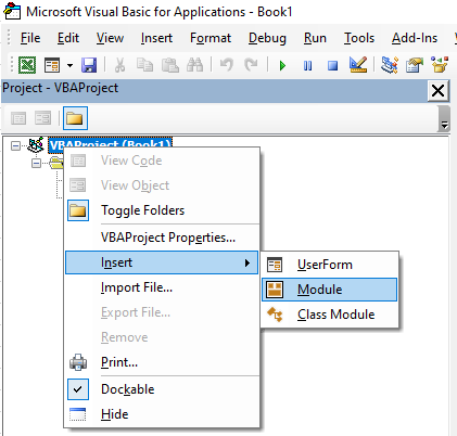
    3. In the top menu bar of the editor, click Insert ➔ Module. A blank white code window will appear.

    Step 2: Copy and Paste the VBA Code

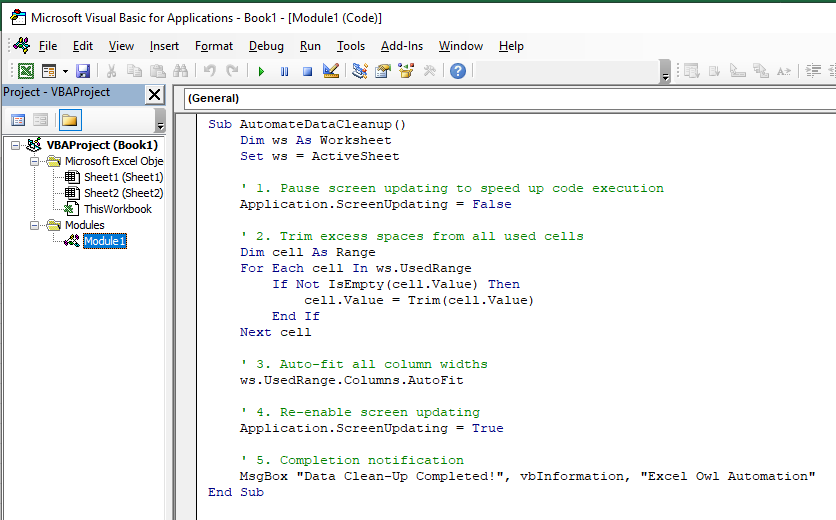
    Copy the ENTIRE code block below (from Sub down to End Sub) and paste it directly into the blank module window:

    Sub AutomateDataCleanup()
        Dim ws As Worksheet
        Set ws = ActiveSheet
        
        ' 1. Pause screen updating to speed up code execution
        Application.ScreenUpdating = False
        
        ' 2. Trim excess spaces from all used cells
        Dim cell As Range
        For Each cell In ws.UsedRange
            If Not IsEmpty(cell.Value) Then
                cell.Value = Trim(cell.Value)
            End If
        Next cell
        
        ' 3. Auto-fit all column widths
        ws.UsedRange.Columns.AutoFit
        
        ' 4. Re-enable screen updating
        Application.ScreenUpdating = True
        
        ' 5. Completion notification
        MsgBox "Data Clean-Up Completed!", vbInformation, "Excel Owl Automation"
    End Sub

    Step 3: Run the Macro Using Alt + F8 Shortcut

    You don’t need to open the VBA Editor every time you want to clean up your data. You can run your macro directly from your Excel spreadsheet using a quick shortcut:

    1. Switch back to your main Excel sheet window.
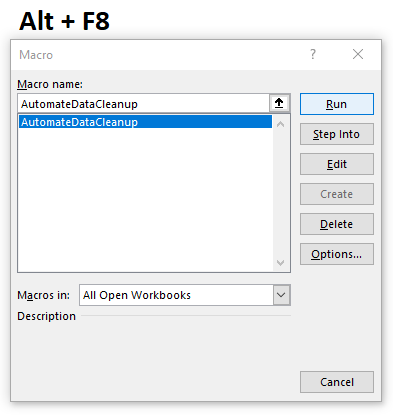
    2. Press Alt + F8 (Option + F8 on Mac) to open the Macro Dialog Box.
    3. Select AutomateDataCleanup from the list of available macros.
    4. Click the Run button on the right.

    💡 Pro Tip: Running directly inside VBA Editor
    If you are still inside the VBA Editor code window, simply place your cursor anywhere inside the code and press F5 (or click the green Run ▶ icon at the top toolbar) to execute it immediately.


    Step 4: Save as Macro-Enabled Workbook (.xlsm)

    To ensure your new macro is preserved when you close Excel, you must save your file in a macro-enabled format:

    1. Click File ➔ Save As (or press F12).
    2. In the Save as type drop-down menu, select Excel Macro-Enabled Workbook (*.xlsm).
    3. Click Save.

    ⚠️ Important Note: Standard .xlsx files cannot store VBA scripts. If you save as a normal .xlsx workbook, your macro code will be permanently deleted!

  • How to Highlight Duplicate Values in Excel in 3 Easy Steps

    Before you permanently delete duplicate rows from a dataset, it is often best practice to visual identify them first. Highlighting duplicates allows you to review repeating entries, spot data entry errors, and verify information without losing any raw data.

    In this quick guide, you will learn how to instantly highlight duplicate values in Excel using Conditional Formatting.


    Why Highlight Duplicates First?

    While Excel’s Remove Duplicates feature permanently deletes repeating rows, highlighting gives you full control:

    • Visual Audit: Instantly scan where repeating entries occur across your sheet.
    • Safer Data Cleaning: Verify whether a duplicate is a genuine error or an acceptable duplicate entry before deleting.
    • Non-Destructive: Highlights can be cleared at any time without altering your actual cell values.

    Step 1: Select Your Data Range

    1. Click and drag to highlight the cells, column, or row you want to check for duplicate values.
    2. To select an entire column, click the column letter header at the top (e.g., Column A).
    3. To select a specific table range, press Ctrl + A while inside the dataset.

    Tip: If you only want to highlight duplicates within a specific column (such as Email Addresses or Customer IDs), select only that specific column.


    Step 2: Apply Conditional Formatting

    1. Navigate to the Home tab on the Excel Ribbon.
    2. In the Styles group, click Conditional Formatting.
    3. Hover over Highlight Cells Rules and select Duplicate Values… from the sub-menu.

    Step 3: Choose Your Highlight Color and Confirm

    1. A dialog box will appear. Ensure the first drop-down menu is set to “Duplicate” (not “Unique”).
    2. In the second drop-down menu, choose your preferred formatting style (e.g., Light Red Fill with Dark Red Text).
    3. Click OK.

    Excel will immediately scan your selected range and highlight every repeating value!


    How to Clear the Duplicate Highlights

    When you are done reviewing your data, removing the color highlights takes just two clicks:

    1. Select your data range again.
    2. Go to Home ➔ Conditional Formatting ➔ Clear Rules ➔ Clear Rules from Selected Cells.

    Summary

    Using Conditional Formatting to highlight duplicates is one of the simplest yet most effective data validation techniques in Excel. Combine this visual check with Excel’s built-in Remove Duplicates tool to ensure your spreadsheets remain accurate and error-free.

  • How to Unpivot Data in Excel in 3 Easy Steps (Power Query)

    When working with data in Excel, you often encounter crosstab reports—tables where dates or categories are spread across columns rather than rows. While these wide tables are easy for humans to read, they are difficult to analyze using Pivot Tables or formulas.

    In this guide, you will learn how to quickly convert wide data into a flat, tabular format using Excel’s built-in Power Query tool without writing any complex formulas.


    Why Should You Unpivot Data?

    Unpivoting transforms a wide table into a tall, structured format with normalized columns:

    • Before: Columns for Jan, Feb, Mar, Apr.
    • After: One column for Month and one column for Sales.

    This format is required for building dynamic Pivot Tables, dashboards, and automated reporting workflows.


    Step 1: Import Your Data into Power Query

    1. Select any cell inside your dataset.
    2. Go to the Data tab on the Excel Ribbon.
    3. Click From Sheet (or From Table/Range in older versions).
    4. In the pop-up dialog, ensure your data range is correct and check “My table has headers.” Click OK.

    Note: This opens the Power Query Editor window, leaving your original raw data safe and untouched.


    Step 2: Unpivot the Columns

    1. In the Power Query Editor, click on the primary identifier column (e.g., Product ID or Category).
    2. Right-click the column header.
    3. Select Unpivot Other Columns.

    Excel will instantly stack all remaining columns into two simple columns: Attribute and Value.


    Step 3: Rename Columns and Load to Excel

    1. Double-click the Attribute column header and rename it to Month (or Period).
    2. Double-click the Value column header and rename it to Sales (or Amount).
    3. Click the Close & Load button in the top-left corner of the Home tab.

    Power Query will output the clean, transformed data onto a brand-new worksheet!


    Summary

    Unpivoting data is one of the most powerful features in Excel’s toolset. Instead of spending hours manually copying and transposing cells, Power Query allows you to automate data cleanup in seconds with just three clicks.

  • How to Remove Duplicate Rows in Excel in 3 Easy Steps

    How to Remove Duplicate Rows in Excel in 3 Easy Steps

    Dealing with duplicate data is one of the most common headaches when handling spreadsheets. Whether you are cleaning up a contact list or preparing a sales report, duplicate records can lead to inaccurate calculations and messy reports.

    Fortunately, Excel provides a built-in feature to remove duplicates in just a few clicks—without using complex formulas or scripts.

    Here is a step-by-step guide to cleaning up your dataset instantly.


    Step 1: Select Your Data Range

    1. Open your Excel worksheet and click any cell within your data table.
    2. If you want to clean the entire table, press Ctrl + A to select all data.
    3. If you only want to check specific columns, highlight those columns directly.

    💡 Quick Tip: Make sure your table has clear column headers (e.g., Name, Email, ID) before moving to the next step.


    Step 2: Open the ‘Remove Duplicates’ Tool

    1. Navigate to the Data tab on the top ribbon menu.
    2. In the Data Tools group, click on Remove Duplicates.
    3. A popup dialog box will appear on your screen.

    Step 3: Choose Columns and Remove Duplicates

    1. In the popup window, check the box that says “My data has headers” (if your table includes header titles).
    2. Select the columns you want Excel to inspect for duplicates:
    • Exact Row Match: Keep all columns checked if you want to delete rows where every single field is identical.
    • Key Field Match: Check only specific columns (e.g., Email or Customer ID) if you want to remove duplicates based on a unique identifier.
    1. Click OK.

    Excel will instantly process your data and display a message showing how many duplicate values were found and removed, along with the count of remaining unique values.


    Summary Checklist

    • Shortcut to Select All: Ctrl + A
    • Menu Path: Data TabRemove Duplicates
    • Best Practice: Always save a backup copy of your original file before deleting duplicate rows.
  • How to Fix Excel Error Codes (#N/A, #VALUE!, #####) in 5 Minutes

    When working in Excel, suddenly seeing messy error codes like ####, #N/A, or #VALUE! can trigger instant panic—especially right before submitting an important report. Don’t worry; Excel errors are just helpful warning signs that something in your formula or data needs a minor adjustment. Once you know the cause, you can fix them in under 5 minutes.

    This guide breaks down the 5 most common Excel errors in the workplace and shows you how to resolve them quickly.


    1. When Column Width is Too Narrow: ##### Error

    • Cause: This isn’t actually a formula error. It happens when the column isn’t wide enough to display all the digits of a number or date.
    • Fix: Double-click the right boundary of the column header or drag it wider to reveal the data instantly.

    2. When a Lookup Value Cannot Be Found: #N/A Error

    • Cause: Functions like VLOOKUP, XLOOKUP, or MATCH return this error when they cannot find an exact match for your lookup value within the specified range.
    • Fix:
      • Check for typos, hidden spaces, or mismatched data types in your lookup criteria.
      • Wrap your formula inside an IFERROR function to display a clean alternative instead of an error.
      • Example formula: =IFERROR(VLOOKUP(A2, B:C, 2, FALSE), "Not Found")

    3. When Data Types Don’t Match: #VALUE! Error

    • Cause: This happens when you try to perform mathematical operations on incompatible data types, such as adding text (“abc”) to a number.
    • Fix:
      • Verify the data types of all cells involved in your calculation.
      • Check for hidden leading or trailing spaces that might be turning numbers into text strings.

    4. When a Formula Name is Misspelled: #NAME? Error

    • Cause: Excel displays this when it doesn’t recognize a function name due to a typo, or when you forget to enclose text strings in quotation marks ("").
    • Fix:
      • Double-check your spelling (e.g., make sure VLOOKUP isn’t typed as VLCKUP).
      • Ensure any literal text inside formulas uses proper double quotes.

    5. When Division by Zero Occurs: #DIV/0! Error

    • Cause: This error pops up when a formula attempts to divide a number by zero or by an empty cell.
    • Fix:
      • Check the divisor cell to ensure it contains a valid non-zero number.
      • Use IFERROR to return zero or a blank space when a division error happens.
      • Example formula: =IFERROR(A1/B1, 0)

    Excel error codes are simply friendly road signs telling you a formula needs a quick tune-up. By staying calm and applying a handy wrapper like IFERROR, you can keep your spreadsheets looking pristine and professional!

  • Excel VLOOKUP Function Guide: Basic Usage and XLOOKUP Comparison

    When working with relational data across different sheets or tables, retrieving matching information manually is nearly impossible. For decades, VLOOKUP has been the industry-standard function for cross-referencing data in Excel.

    However, Microsoft introduced XLOOKUP in modern versions of Excel to address long-standing limitations of VLOOKUP. In this guide, we cover how VLOOKUP works step-by-step, common errors to avoid, and why transitioning to XLOOKUP will save you hours of work.


    💼 Real-World Scenario: When Do You Need Lookup Functions?

    Suppose you have an Employee ID list in Sheet A and a master Salary Database in Sheet B. Instead of searching each Employee ID manually, a lookup formula searches the ID in Sheet B and automatically retrieves the corresponding salary into Sheet A.


    🔍 Part 1: How VLOOKUP Works (Step-by-Step)

    VLOOKUP stands for Vertical Lookup. It searches for a specific value in the first column of a table and returns a value in the same row from a specified column to the right.

    Syntax

    “`excel
    =VLOOKUP(lookup_value, table_array, col_index_num, [range_lookup])

  • How to Create a Pivot Table in Excel: A Step-by-Step Data Analysis Guide

    Analyzing thousands of rows of raw transactional data manually is time-consuming and prone to human error. Pivot Tables are one of Excel’s most powerful built-in tools, allowing you to summarize, aggregate, and explore massive datasets in just a few clicks—without writing a single formula.

    In this step-by-step guide, we will walk through how to build a Pivot Table from scratch, apply key filters, and troubleshoot common formatting issues.


    💼 Real-World Scenario: Why Use a Pivot Table?

    Imagine you have a sales log containing 5,000 rows with columns for Date, Region, Sales Rep, Product, and Revenue.

    • Without Pivot Tables: You would need to use complex SUMIFS or COUNTIFS formulas to calculate total revenue per region or per sales rep.
    • With Pivot Tables: You simply drag and drop fields into four distinct areas to instantly calculate totals, averages, and percentage breakdowns.

    🛠️ Step 1: Preparing Your Source Data

    Before inserting a Pivot Table, ensure your source dataset adheres to these 3 strict rules:

    1. Unique Column Headers: Every column must have a clear, non-blank header name in the top row.
    2. No Empty Rows or Columns: Ensure there are no completely blank rows or columns splitting your dataset.
    3. No Merged Cells: Unmerge all merged cells within the data range.

    💡 Pro Tip: Convert your raw data range into an official Excel Table (Ctrl + T) before creating a Pivot Table. This ensures that any new rows added later will automatically be included when you refresh the Pivot Table!


    🚀 Step 2: Creating the Pivot Table

    1. Click any single cell inside your data dataset.
    2. Go to the Insert tab on the ribbon menu and click PivotTable.
    3. In the pop-up dialog, verify that your data range is selected correctly.
    4. Choose New Worksheet as the destination and click OK.

    🧭 Step 3: Understanding the 4 Pivot Table Fields

    A new worksheet will open with an empty Pivot Table grid on the left and the PivotTable Fields pane on the right. You can drag your column names into four areas:

    AreaPurposeExample Usage
    FiltersRestricts top-level data across the entire tableFilter by Year or Status
    ColumnsDisplays selected field values across horizontal headersDisplay Region (East, West, North) across top
    RowsDisplays selected field values down vertical rowsList Sales Rep names vertically
    ValuesPerforms numeric calculations (Sum, Count, Average)Calculate total Revenue

    🔧 Step 4: Formatting Numeric Values

    By default, Pivot Tables display unformatted numbers (e.g., 1250000). To apply currency or thousands commas cleanly across the entire summarized field:

    1. Right-click any numeric cell inside the Pivot Table values.
    2. Select Number Format… (Do NOT choose Format Cells).
    3. Select Number or Currency, check Use 1000 Separator (,), and click OK.

    ⚠️ Troubleshooting Common Pivot Table Errors

    1. Values Display as “Count of Revenue” Instead of “Sum of Revenue”

    • Cause: Your source data column contains at least one blank cell or text entry.
    • Solution: Right-click the header ➔ Select Summarize Values By ➔ Change from Count to Sum.

    2. New Data Added to Source Range Does Not Appear

    • Cause: Pivot Tables do not auto-refresh when source data changes.
    • Solution: Right-click inside the Pivot Table and click Refresh (or press Alt + F5).

    Conclusion

    Pivot Tables transform raw transactional logs into actionable business summaries within seconds. Mastering drag-and-drop fields and numeric formatting will elevate your analytical capability immediately.

    In our next guide, we will explore Excel VLOOKUP Function Guide: Basic Usage and XLOOKUP Comparison to master cross-referencing data across multiple tables!

  • Mastering Excel Cell Formatting (Ctrl + 1): Quick Guide for Beginners

    Have you ever typed a date into Excel only to see it turn into a strange number like 45442? Or spent extra time manually typing currency symbols or units like “USD”, “pcs”, or “lbs” next to every number?

    All these issues can be resolved in seconds once you understand Cell Formatting using the shortcut Ctrl + 1. In this guide, we cover 3 essential cell formatting techniques every Excel user should know.


    1. Apply Thousands Separators (,) and Currency Formats

    Large numbers without commas are difficult to read. You can format numbers cleanly in just a few clicks.

    1. Select the range of cells containing the numbers.
    2. Press Ctrl + 1 to open the Format Cells dialog box.
    3. Navigate to [Number] ➔ [Number] in the Category menu.
    4. Check the box for ‘Use 1000 Separator (,)’ and click OK.

    💡 Quick Tip: You can also click the Comma Style (,) button directly in the Home tab on the ribbon menu!


    2. Append Custom Units (“USD”, “pcs”, “items”) Automatically

    If you manually type text alongside numbers in a cell (e.g., 100 pcs), Excel treats the cell as Text, which prevents functions like SUM or AVERAGE from calculating properly!

    To keep numeric properties intact for calculations while displaying custom units on screen, use Custom Formatting:

    1. Press Ctrl + 1 ➔ Go to [Number] tab ➔ Click [Custom].
    2. In the Type input box on the right, enter one of these formatting codes:
    • #,##0" USD" ➔ Formats with thousands commas and appends ‘USD’ (e.g., 1,000,000 USD)
    • #,##0" pcs" ➔ Appends quantity units (e.g., 50 pcs)
    • 0000 ➔ Pads leading zeros to match a fixed digit length (e.g., entering 5 displays as 0005)

    3. Fix Corrupted or Numeric Date Displays

    When entering dates, you might occasionally see raw serial numbers like 46225 instead of 2026-07-22. This happens because Excel calculates dates as sequential serial numbers starting from January 1, 1900.

    • How to Fix: Select the cells ➔ Press Ctrl + 1 ➔ Choose [Date] ➔ Select your preferred date format (e.g., YYYY-MM-DD or MM/DD/YYYY).

    📊 High-Yield Custom Formatting Codes for Daily Use

    Raw DataCustom Format CodeDisplayed ResultPractical Description
    1234567#,##01,234,567Standard thousands separator
    1234567#,##0" USD"1,234,567 USDThousands separator + currency suffix
    50#,##0" pcs"50 pcsQuantity suffix (retains formula usability)
    202607220000-00-002026-07-22Formats 8-digit numbers as standard dates

    Conclusion

    Mastering Cell Formatting dramatically improves data readability and prevents formula errors before they happen.

    This concludes our essential Basics series (Shortcuts, Formulas, and Formatting)!

    Starting with our next post, we will move into the Tools category to explore powerful productivity features: Pivot Tables and VLOOKUP / XLOOKUP functions.